Chapter 15 Waves-I

Learning Objectives:

In this chapter you will basically learn:

\(\bullet\) How to identify the three main types of waves.

\(\bullet\) Distinguishing between transverse waves and longitudinal waves.

\(\bullet\) How to determine amplitude , angular wave number k, angular frequency v, phase constant f, and direction of travel, and calculate the phase \((kx \pm \omega t + \phi)\) and the displacement at any given time and position.

\(\bullet\) Know the relation between the wave speed v, the distance traveled by the wave, and the time required for that travel.

\(\bullet\) Know the relationships between wave speed v, angular frequency \(\omega\), angular wave number k, wavelength \(\lambda\), period T, and frequency f.

\(\bullet\) Calculate the transverse velocity u(t), transverse acceleration a(t) of a string element as a transverse wave moves through its location.

\(\bullet\) Calculate the linear density m of a uniform string in terms of the total mass and total length.

\(\bullet\) Apply the relationship between wave speed v, tension \(\tau\), and linear density \(\mu\).

\(\bullet\) Calculate the average rate at which energy is transported by a transverse wave.

\(\bullet\) Apply the principle of superposition to show that two overlapping waves add algebraically to give a resultant (or net) wave.

\(\bullet\) Describe how the phase difference between two transverse waves (with the same amplitude and wavelength) can result in fully constructive interference, fully destructive interference, and intermediate interference.

\(\bullet\) Sketch a phasor diagram for two overlapping waves traveling together on a string, indicating their amplitudes and phase difference on the sketch.

\(\bullet\) By using phasors, find the resultant wave of two transverse waves traveling together along a string, calculating the amplitude and phase and writing out the displacement equation, and then displaying all three phasors in a phasor diagram that shows the amplitudes, the leading or lagging, and the relative phases.

\(\bullet\) For two overlapping waves (same amplitude and wavelength) that are traveling in opposite directions, sketch snapshots of the resultant wave, indicating nodes and antinodes.

\(\bullet\) For a string element at an antinode of a standing wave, write equations for the displacement, transverse velocity, and transverse acceleration as functions of time.

15.1 Types of Waves:

Waves are of three main types:

1. Mechanical waves: These waves are most familiar because we encounter them almost constantly; common examples include water waves, sound waves, and seismic waves. All these waves have two central features: They are governed by Newton’s laws, and they can exist only within a material medium, such as water, air, and rock.

2. Electromagnetic waves: These waves are less familiar, but you use them constantly; common examples include visible and ultraviolet light, radio and television waves,microwaves, x rays, and radar waves.These waves require no material medium to exist. Light waves from stars, for example, travel through the vacuum of space to reach us. All electromagnetic waves travel through a vacuum at the same speed c = 299 792 458 m/s.

3. Matter waves: Although these waves are commonly used in modern technology, they are probably very unfamiliar to you. These waves are associated with electrons, protons, and other fundamental particles, and even atoms and molecules. Because we commonly think of these particles as constituting matter, such waves are called matter waves.

15.2 Transverse and Longitudinal Mechanical Waves:

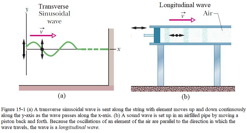
In a transverse mechanical wave the displacement of the oscillating string element is perpendicular to the direction of travel of the wave, as shown in Fig. 15-1a. In this Chapter 15 we focus on transverse waves, and string waves in particular; in Chapter 16 we focus on longitudinal waves, and sound waves in particular.

Fig. 15-1b shows how a sound wave can be produced by a piston in a long, air-filled pipe is called Longitudinal Waves. The motion of the elements of air is parallel to the direction of the wave’s travel, the motion is said to be longitudinal, and the wave is said to be a longitudinal wave.

15.3 Wavelength and Frequency of Transverse Wave:

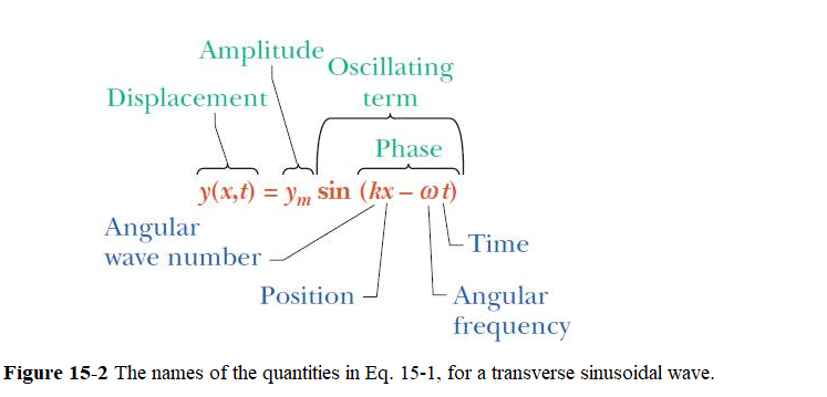
We can formulate a sinusoidal wave like that of Fig. 15-1a traveling in the positive direction of an x axis. As the wave moves through succeeding elements (that is, very short sections) of the string, the elements oscillate along to the y axis. At time t, the displacement y of the element located at position x is given by

\[\begin{equation} y(x,t)=y_m\sin(kx-\omega t). \tag{15.1} \end{equation}\]

The names of the quantities in Eq. 15-1 are shown in Fig. 15-2.

Amplitude and Phase:

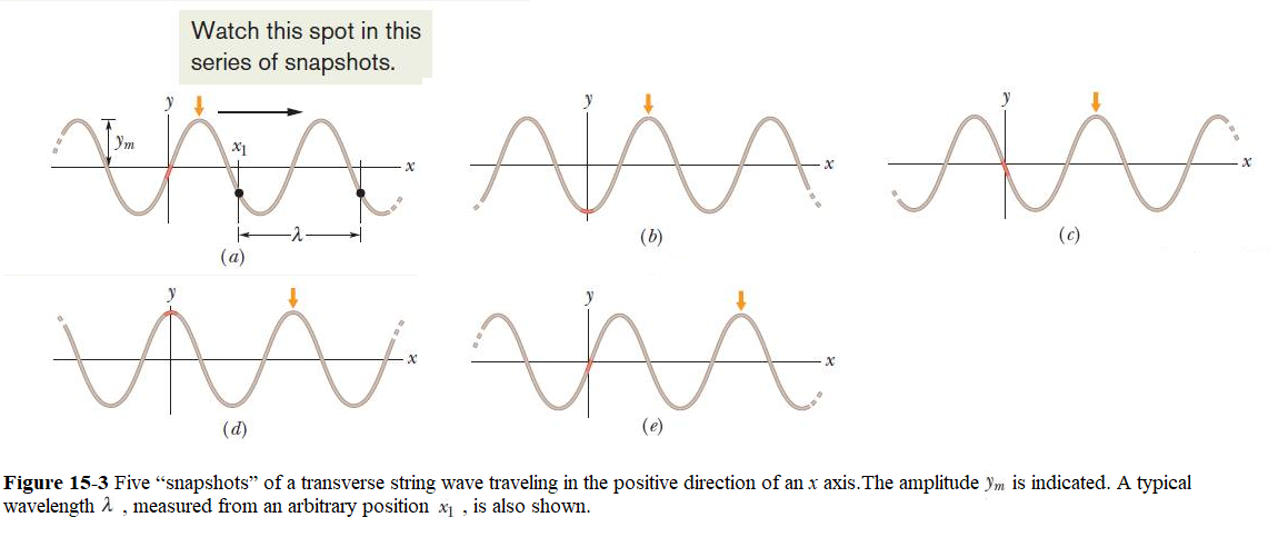
The amplitude \(y_m\) of a wave, as shown in Fig. 15-3 , is the magnitude of the maximum displacement of the elements from their equilibrium positions as the wave passes through them. (The subscript m stands for maximum.)

Since \(y_m\) is a magnitude, if it is measured downward instead of upward as drawn in Fig. 15-3a, it is considered to be positive.

The phase of the wave is the argument \((kx - \omega t)\) of the sine wave in Eq. 15-1. As the wave sweeps through a string element at a particular position x, the phase changes linearly with time t. This means that the sine also changes, oscillating between +1 and -1. Its extreme positive value (+1) corresponds to a peak of the wave moving through the element; at that instant the value of y at position x is \(y_m\). Its extreme negative value (-1) corresponds to a valley of the wave moving through the element; at that instant the value of y at position x is \(-y_m\). Therefore, the sine function and the time-dependent phase of a wave correspond to the oscillation of a string element, and the amplitude of the wave determines the extremes of the element’s displacement of a transverse wave in a string.

Wavelength and Angular Wave Number:

The wavelength \(\lambda\) of a wave is the distance (parallel to the direction of the wave’s travel) between repetitions of the shape of the wave (or wave shape).

A typical wavelength is marked in Fig. 15-3a, which is a snapshot of the wave at time t = 0. So, at the instant t = 0, Eq. 15-1 gives the following equation,

\[\begin{equation} y(x,0)=y_m\sin(kx). \tag{15.2} \end{equation}\]

Due to periodic property of sine wave, the displacement y is the same at \(x = x_1\) and \(x = x_1 + \lambda\). From Eq. 16-2, we can get

\[\begin{equation} y_m\sin(kx_1)=y_m\sin k(x_1+\lambda)=y_m\sin(kx_1+k\lambda). \tag{15.3} \end{equation}\]

A sine function begins to repeat itself when its angle (or argument) is increased by \(2\pi\) rad, so in Eq. 15-3 we must have \(k\lambda = 2\pi\), so the angular wave number is

\[\begin{equation} k = \frac{2\pi}{\lambda}~~~(angular~ wave~ number). \tag{15.3} \end{equation}\]

The angular wave number k and its SI unit is the radian per meter, or the inverse meter. (The symbol k for angular wave number not to be confused with k of the spring constant as used previously.)

Period, Angular Frequency, and Frequency:

Now consider the displacement y of Eq. 15-1 as function of t at a certain position along the string, taken to be x = 0 as can be seen in Figure 15-4.

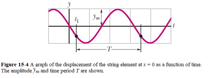
\[\begin{equation} y(0,t) = -y_m\sin\omega t~~~~(x=0). \tag{15.4} \end{equation}\]

Where we have made use of the fact that sine function is an odd function for which \(\sin(-\omega t) = -\sin(\omega t)\).

We define the period of oscillation T of a wave to be the time the string element moves through one full cycle. A typical period is marked on the graph of Fig. 16-5. Applying Eq. 15-4 to both ends of this time interval and equating the results yield

\[\begin{equation} -y_m\sin(\omega t_1)=-y_m\sin(\omega t_1+\omega T). \tag{15.5} \end{equation}\]

To hold the equality in Eq. 15-5, it is required to have \(\omega T = 2pi\), or if

\[\begin{equation} \omega = \frac{2\pi}{T}~~~(angular~frequency). \tag{15.6} \end{equation}\]

Here, \(\omega\) is called the angular frequency of the wave with it’s SI unit is the radian per second.

The frequency f of a wave is defined as 1/T and is related to the angular frequency \(\omega\) by

\[\begin{equation} f = \frac{1}{T}=\frac{\omega}{2\pi}~~~(frequency). \tag{15.7} \end{equation}\]

The SI unit of f is usually measured as the number of oscillations per unit time and is called hertz (Hz).

15.4 The Speed of a Traveling Wave:

Figure 15-5 shows two snapshots of the wave of Eq. 15-1, taken a small time interval \(\Delta t\) apart. The wave is traveling in the positive direction of x (to the right in Fig. 15-5), the entire wave pattern moving a distance \(\Delta x\) in that direction during the interval \(\Delta t\). The ratio \(\frac{\Delta x}{\Delta t}\) (or, in the differential limit, dx/dt) is the wave speed v. How can we find its value?

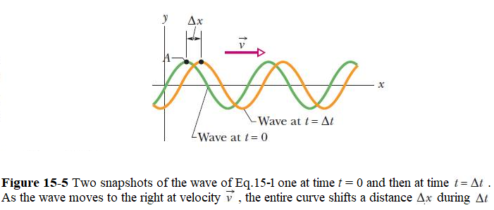
Considering a point A retains its displacement as it moves, the phase in Eq.15-1 giving it that displacement must remain a constant:

\[\begin{equation} kx - \omega t = a ~constant. \tag{15.8} \end{equation}\]

Taking derivative of both sides of Eq. 15-8, we get

\[\begin{equation} k\frac{dx}{dt} - \omega \frac{dt}{dt} = \frac{d (a~ constant)}{dt}=0. \end{equation}\]

or

\[\begin{equation} v=\frac{dx}{dt} = \frac{\omega}{k}. \tag{15.9} \end{equation}\]

Thus, a wave traveling in the postitive direction of x is described by the Eq. 15-1.

Making use of Eq. 15-3 \((k =\frac {2\pi}{\lambda})\) and Eq. 15-6 \((\omega = \frac{2\pi}{T})\), we can rewrite wave speed in Eq. 15-9 as

\[\begin{equation} v=\frac{\omega}{k}=\frac{\frac{2\pi}{T}}{\frac{2\pi}{\lambda}}=\frac{\lambda}{T}=\lambda f. \tag{15.10} \end{equation}\]

We can find the equation of a wave traveling in the negative direction of x by replacing t in Eq. 15-2 with \(-t\).This corresponds to the condition

\[\begin{equation} kx + \omega t = a ~constant. \tag{15.11} \end{equation}\]

\[\begin{equation} k\frac{dx}{dt} + \omega \frac{dt}{dt} = \frac{d (a~ constant)}{dt}=0. \end{equation}\]

or

\[\begin{equation} v=\frac{dx}{dt} = -\frac{\omega}{k}. \tag{15.12} \end{equation}\]

Thus, a wave is traveling in the negative direction of x in Eq. 15-12. Thus, a wave traveling in the negative direction of x is described by modifying Eq. 15-1

\[\begin{equation} y(x,t)=y_m\sin(kx+\omega t). \tag{15.13} \end{equation}\]

15.5 Wave Speed on a Stretched String:

Consider a single symmetrical pulse such as that of Fig. 15-6, moving from left to right along a string with speed v. In a reference frame in which the pulse remains stationary, the string appears to move past us, from right to left in Fig. 15-6, with speed v.

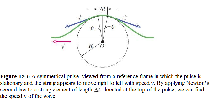
Consider a small string element of length \(\Delta l\) within the pulse, an element that forms an arc of a circle of radius R and subtending an angle \(2\theta\) at the center of that circle. The tension in the string \(\vec\tau\) with its components pulls tangentially on this element at each end. The horizontal components of these forces cancel each other, but the vertical components add to form a radial restoring force \(\vec F\). In magnitude,

\[\begin{equation} F = 2(\tau\sin\theta)\approx \tau(2\theta)=\tau\frac{\Delta l}{R}~~~(force). \tag{15.8} \end{equation}\]

\[\begin{equation} F = \tau\frac{\Delta l}{R}= ma = (\mu\Delta l)\frac{v^2}{R}. \tag{15.9} \end{equation}\]

\[\begin{equation} v = \sqrt{\frac{\tau}{\mu}} \tag{15.10} \end{equation}\]

where \(\mu=\frac{\Delta m}{\Delta l}\) is the linear mass density.

15.6 Energy and Power of a Wave Traveling Along a String:

The kinetic energy dK associated with a string element of mass dm is given by

\[\begin{equation} dK = \frac{1}{2}dm~u^2 \tag{15.14} \end{equation}\]

where u is the transverse speed of the oscillating string element. To find u, we differentiate Eq. 16-1 with respect to time while holding x constant:

\[\begin{equation} u = \frac{\partial y}{\partial t} = -\omega y_m \cos(kx-\omega t). \tag{14.30} \end{equation}\]

Using \(dm = \mu dx\), we rewrite Eq. 15-14 as

\[\begin{equation} dK = \frac{1}{2}dm~u^2=\frac{1}{2}(\mu dx)(-\omega y_m)^2\cos^2(kx-\omega t). \tag{15.15} \end{equation}\]

Dividing Eq. 15-16 by dt gives the rate at which kinetic energy passes through a string element, and thus the rate at which kinetic energy is carried along by the wave. The dx/dt that then appears on the right of Eq. 15-16 is the wave speed v, so

\[\begin{equation} \frac{dK}{dt} =\frac{1}{2}\mu v\omega^2 y_m^2\cos^2(kx-\omega t) \tag{15.16} \end{equation}\]

The average rate at which kinetic energy is transported is

\[\begin{equation} \left(\frac{dK}{dt}\right)_{avg} =\frac{1}{2}\mu v\omega^2 y_m^2\left[\cos^2(kx-\omega t)\right]_{avg}=\frac{1}{4}\mu v\omega^2 y_m^2 \tag{15.17} \end{equation}\]

The average value of the square of a cosine function over an integer number of periods is \(\frac{1}{2}\).

The average power, which is the average rate at which energy of both kinds is transmitted by the wave, is then

\[\begin{equation} P_{avg} = 2\left(\frac{dK}{dt}\right)_{avg}=\frac{1}{2}\mu v\omega^2 y_m^2~~~(average~power). \tag{15.18} \end{equation}\]

The factors m and v in this equation depend on the material and tension of the string. The factors v and \(y_m\) depend on the process that generates the wave.The dependence of the average power of a wave on the square of its amplitude and also on the square of its angular frequency is a general result, true for waves of all types.

15.7 Interference of Waves:

Interference of waves happens when we send two or more sinusoidal waves propagate along a stretched string with their respective amplitudes and wavelengths. Using superposition principle of waves we can find the resultant wave of the incident waves.

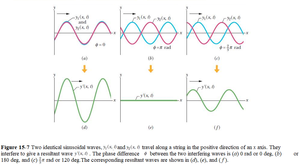
Let us consider two waves with same wavelength and amplitude but the second wave is shifted by a phase difference of \(\phi\) traveling along a stretched string be given by

\[\begin{equation} y_1(x,t)=y_m\sin(kx-\omega t) \tag{15.19} \end{equation}\]

and

\[\begin{equation} y_2(x,t)=y_m\sin(kx-\omega t+\phi). \tag{15.20} \end{equation}\]

By applying the superposition principle the resultant wave is the algebraic sum of the two waves as follows

\[y'(x,t)=y_1(x,t)+y_2(x,t)\] \[\begin{equation} = y_m\sin(kx-\omega t)+ y_m\sin(kx-\omega t+\phi). \tag{15.21} \end{equation}\]

Using trigonometric identity as given in Appendix-A for two sine waves with angles \(\alpha\) and \(\beta\) as

\[\begin{equation} \sin\alpha + \sin\beta = 2\sin\frac{1}{2}(\alpha+\beta)\cos\frac{1}{2}(\alpha-\beta), \tag{15.22} \end{equation}\]

Eq. 15-22 reduces to

\[\begin{equation} y'(x,t) = \left[2y_m\cos\frac{1}{2}\phi\right]\sin(kx-\omega t+\frac{1}{2}\phi). \tag{15.23} \end{equation}\]

The resultant wave in Eq.15-24 has a new amplitude \(y_m'=\left[2y_m\cos\frac{1}{2}\phi\right]\) and has a new phase of \(\frac{1}{2}\phi.\)

The two waves are shown in Fig. 16-14a-c, and their corresponding resultant wavea are shown in Fig. 16-14d-f.

15.8 Phasors:

A phasor is a vector that rotates around its tail, which is pivoted at the origin of a coordinate system.The magnitude of the vector is equal to the amplitude ym of the wave that it represents.The angular speed of the rotation is equal to the angular frequency v of the wave. For example, the wave

\[\begin{equation} y_1(x,t) = y_{m1}\sin(kx-\omega t). \tag{15.24} \end{equation}\]

is represented by the phasor shown in Figs. 15a to d.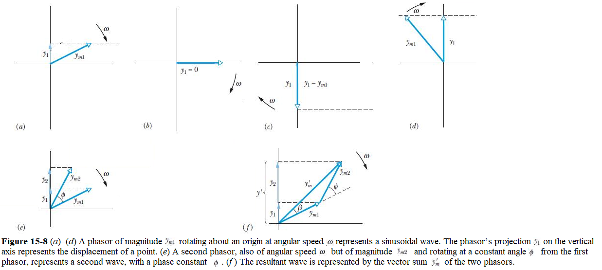 

The magnitude of the phasor is the amplitude \(y_{m1}\) of the wave. As the phasor rotates around the origin at angular speed \(\omega\), its projection \(y_1\) on the vertical axis varies sinusoidally, from a maximum of \(y_{m1}\) through zero to a minimum of \(-y_{m1}\) and then back to \(y_{m1}\). This variation corresponds to the sinusoidal variation in the displacement \(y_1\) of any point along the string as the wave passes through that point.

When two waves travel along the same string in the same direction, we can represent them and their resultant wave in a phasor diagram. The phasors in Fig. 15-8e represent the wave of Eq. 15-25 and a second wave given by

\[\begin{equation} y_2(x,t) = y_{m2}\sin(kx-\omega t+\phi). \tag{15.25} \end{equation}\]

Standing Waves:

In section15-7 we have studied interference of two sinusoidal waves of the same wavelength and amplitude traveling in the same direction along a stretched string. What if they travel in opposite directions? We can again find the resultant wave by applying the superposition principle.

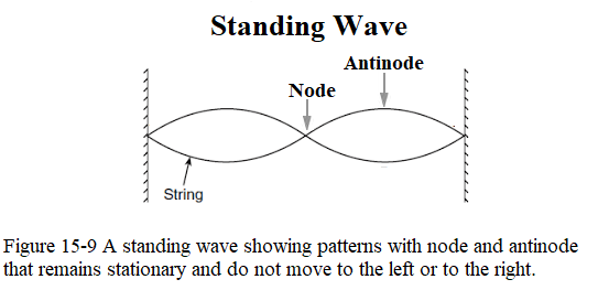
The outstanding feature of the resultant wave is that there are places along the string, called nodes, where the string never moves. Halfway between adjacent nodes are antinodes, where the amplitude of the resultant wave is a maximum. Wave pattern as shown in Fig. 15-9 is called standing waves because the wave patterns do not move left or right; the locations of the maxima and minima do not change.

To analyze a standing wave, we represent the two waves with the equations

\[\begin{equation} y_1(x,t) = y_m\sin(kx-\omega t+\phi) \tag{15.26} \end{equation}\]

and

\[\begin{equation} y_2(x,t) = y_m\sin(kx+\omega t). \tag{15.27} \end{equation}\]

The principle of superposition gives, for the combined wave,

\[\begin{equation} y'(x,t)=y_1(x,t)+y_2(x,t) = y_m\sin(kx-\omega t)+y_m\sin(kx+\omega t). \tag{15.28} \end{equation}\]

Applying the trigonometric relation of Eq. 15-23 we can get

\[\begin{equation} y'(x,t) = \left[2y_m\sin(kx\right]\cos(\omega t). \tag{15.29} \end{equation}\]

In the standing wave of Eq. 15-30, the amplitude is zero for values of kx that give \(\sin kx = 0\).Those values are

\[\begin{equation} kx = n\pi, ~for~n =0,1,2,...... \tag{15.30} \end{equation}\]

Substituting \(k = \frac{2\pi}{\lambda}\) in Eq. 15-31 and rearranging, we get

\[\begin{equation} x = n\frac{\lambda}{2}, ~for~n =0,1,2,....(nodes), \tag{15.31} \end{equation}\]

as the positions of zero amplitude—the nodes—for the standing wave of Eq. 15-30. Note that adjacent nodes are separated by l/2, half a wavelength. The amplitude of the standing wave of Eq. 15-30 has a maximum value of \(2y_m\),which occurs for values of kx that give \(|\sin kx| = 1\).Those values are

\[\begin{equation} kx = \frac{1}{2}\pi,\frac{3}{2}\pi,\frac{5}{2}\pi,....=\left(n+\frac{1}{2}\right)\pi,~for~n =0,1,2,..., \tag{15.32} \end{equation}\]

Substituting \(k = \frac{2\pi}{\lambda}\) in Eq. 15-33 and rearranging, we get

\[\begin{equation} x = \left(n+\frac{1}{2}\right)\frac{\lambda}{2}, ~for~n =0,1,2,....(antinodes), \tag{15.33} \end{equation}\]

(Solved Problems : 9, , 12, 14, 17, 24, 26, 36, 37,41, 45,49, 58)